Cost Function & Gradient Descent in Context of Machine Learning

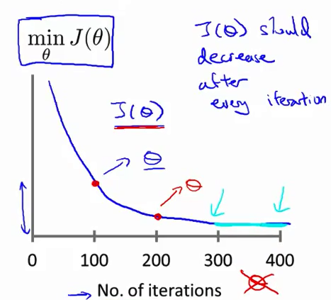
A cost function is something you want to minimize. For example, your cost function might be the sum of squared errors over your training set. 

Gradient descent is a method for finding the minimum of a function of multiple variables. So you can use gradient descent to minimize your cost function. 

If your cost is a function of K variables, then the gradient is the length-K vector that defines the direction in which the cost is increasing most rapidly. So in gradient descent, you follow the negative of the gradient to the point where the cost is a minimum. 

If someone is talking about gradient descent in a machine learning context, the cost function is probably implied (it is the function to which you are applying the gradient descent algorithm).

To Know More Details-

cost Function

Gradient Descent

Logistic Regression in R with and without R library

Logistic Regression with Regularization without using R library

costFunctionReg.R

 costFunctionReg <- function(theta,X,y,lambda){  
  m <- length(y);  
  trunctheta = theta[2:length(theta)]  
  J = -1/m *( sum( y * log(sigmoid(X%*%theta))) + sum((1 - y )*log(1 - sigmoid(X %*% theta))))+(lambda/(2 * m))*sum(trunctheta ^ 2);  
 }  

}

Feature Mapping-

 mapFeature <- function(x1,x2,degree){  
  out <- matrix(1,length(x1));  
  for (i in 1:degree){  
   for (j in 0:i){  
    out <- cbind(out, (x1^(i-j))*(x2^j));  
   }  
  }  
  return(out)  
 }  

sigmoid function

 sigmoid <- function(z) {  
  1/(1 + exp(-z))  
 }  

Predict Function

 # Predictor function  
 predict <- function(theta, X){  
  m <- nrow(X)  
  p <- sigmoid(X%*%theta) > .5  
 }  

entire-

 require(Hmisc);  
 source('sigmoid.R')  
 source('mapFeature.R')  
 source('costFunctionReg.R')  
 source('predict.R')  
 setwd("D:/tmp/mlclass-ex1-005/mlclass-ex2-005/R-Studio/matlab");  
 mydata <- read.table("D:/tmp/mlclass-ex1-005/mlclass-ex2-005/R-Studio/ex2data2.txt",header=FALSE,sep=",")  
 names(mydata) <- c("Microchip Test 1","Microchip Test 2","Accepted");  
 x <- mydata[,1:2];  
 y <- mydata[,3];  
 # Plot data to understand the classification problem  
 plot(x,pch=c(24,3)[y+1],bg='yellow')  
 legend(.8,1,c('y = 1','y = 0'),pch=c(3,23),pt.bg='yellow')  
 x <- mapFeature(x[,1],x[,2],6)  
 #Following as well can be used  
 #x <- mapFeature(mydata$"Microchip Test 1",mydata$"Microchip Test 2",6)  
 initial_theta <- matrix(0,ncol(x));  
 # Contour plot of decision boundary  
 Xbase <- mydata[,1:2]  
 y <- mydata[,3]  
 plot(Xbase,pch=c(24,3)[y+1],bg='yellow')  
 legend(.8,1,c('y = 1','y = 0'),pch=c(3,23),pt.bg='yellow')  
 legend(.85,-0.20,c('BL = 0','B = 1','Y = 20','R = 50','G = 100','GR = 400'),pch=c(3,23),pt.bg='yellow')  
 lambda.array <- c(0,1,20,50,100,150);  
 color.array <- c('black','darkblue','yellow','red','green','gainsboro');  
 # Set regularization parameter lambda to 1  
 lambda = 1;  
 d <- 0;  
 VAT <- numeric(0);  
 for( templambda in lambda.array){  
 d <- d + 1;  
 result <- optim(initial_theta,costFunctionReg,gradFunction,method="BFGS",hessian = FALSE,X=x,y=y,lambda = templambda,control=list(maxit=400));  
 theta <- result$par;  
 p <- predict(theta,x);  
 message('Train Accuracy: ', mean((p == y)) * 100)  
 u <- seq(from=-1, to=1.5, by=.05)  
 v <- u  
 z <- matrix(0,length(u),length(v))  
 for (i in 1:length(u)){  
  for (j in 1:length(v)){  
   z[i,j] = mapFeature(u[i],v[j],6)%*%theta  
  }  
 }  
 contour(u,v,z,nlevels=1,add=T,lwd=2,col=color.array[d],drawlabels=F)  
 }  

The output with various lambda value-

Logistic Regression with Regularization WITH R glm library

 data <- read.table("D:/tmp/mlclass-ex1-005/mlclass-ex2-005/R-Studio/ex2data2.txt",header=TRUE,sep=",")  
 names(data) <- c("test1","test2","accept");  
 head(data)  
 model <- glm(accept ~ test1 + test2 , family = binomial("logit"),data=data )  
 summary(model)  
 plot(model,which=1)  
 plot(predict.glm(model),residuals(model))  
 abline(h=0,lty=2,col="green")  
 in_frame<-data.frame(test1=1.0709,test2=0.10015)  
 #?predict.glm  
 output <- predict.glm(model,newdata=in_frame,type = "response")  
 #Any probability or output value if greater than 0.5 means , its 1 else 0  
 if(output >= 0.5){  
  message(" Success ",output)  
 }else{  
  message(" FAILURE ",output)  
 }  

Machine Learning - 5 (Normalization)

part 4 - Machine Learning - 4

Mean Normalization

The make features approximately zero mean

So the formula derived here is –

Example of Feature Scaling

Consider we have a dataset as follows, need to calculate the normalized feature X₁^(1).

Is Gradient Descent working properly 

To check that gradient descent is working properly, we must verify the value of cost function J(theta) after each iteration.

So to each set of iterations , cost function J(theta) is decreasing and finally it converges to minimize and no more change like from 300 – 400.

Obvious gradient descent not working example

If our gradient descent graph shows like above, it means its not converging with each set of iteration and that means its not working properly. So in the above case, we can assume that alpha is pretty high, we must decrease the learning rate so that baby step would have taken.

·        For sufficiently small learning rate (alpha), J(theta) must decrease with every iteration.

·        But if learning rate is too small, gradient descent may take longer time to converge.

Conclusion:

·        Learning rate is too small, slow convergence.

·        Learning rate is too high, J(theta) may not converge or may not decrease with every iteration. It as well sometimes does slow convergence.

To choose try learning rate – 0.0001, 0.001, 0.01, 0.1, 1.. ….

Deciding Features (param) of a hypothesis\cost function

If we are given with multiple features (parameters), it always doesn’t make sense to use them as it is, we can do lots of other operations on it to make it better features.

Consider the following example-

So now as frontage * depth will give total area, we can derive-

x(land area) = frontage * depth

So now hypothesis,

h_Ɵ(x) = Ɵ₀ + Ɵ₁*x

So by defining new feature, we can define a new better model.

Machine Leaning - 4 (More on Gradient Descent)

part 3 - Machine Learning - 3

Gradient Descent with 2 param Example

If we have training set as follows-

We need to calculate J(0 , 1);

Even we have the training set till m= 4, we can verify h6.

Multiple features in Machine Learning

What if we have multiple features and now all them can derive the result different.

What if we have house size, house number, and number of rooms etc. to determine the price, so now we can assume more precise result and different results as well?

To understand this, we have a set of example-

 

Gradient Descent Algorithm for More than one feature

Gradient Descent Main Algorithm

Gradient Descent Algorithm for Linear Expression Single Dimension

Gradient Descent Algorithm for Linear Expression Multiple Dimension

Mathematical tricks to make Gradient Descent Work Well

SCALING

·        The bottom line about making gradient Descent algorithm to work well is all the dimension\features should have a single scaling, precisely one shouldn’t be declared in sq. Feet and other in CM. Try to make all of them in single scale.

E.g.:

X₁ = Size of house (0 – 2000 feets²)

X₂ = number of bedrooms (1- 5)

So now the X1 will make the Cost Function J very very tall and skinny oval shaped as the range is extremely high and over all the impression will be very congested oval shaped graph.

Now on running gradient descent on such output, it may take long time to reach the global minimum as it needs to travel a long distance to reach there.

So to avoid such scenario we must scale the feature, means make both the features under the same scale, so we derive the following formula which finally result a proper gradient descent on cost Function J graph with circles where finding minimum is easy and faster.

Gradient descent to work better – Limited Range

Always try to keep range of gradient descent features under-

Feature scaling speeds up gradient descent by avoiding much extra iteration that are required when one or more features take on much larger values than the rest.

Machine Learning - 3 ( Gradient Descent)

part 2 - Machine Learning - 2

Gradient Descent

Consider you have above datasets which 2 thetas and to get the min of J(Ɵ1,Ɵ2) , you need to reach to the minimum so gradient descent gives the solution for that. Above is a kind of hill where black and red marks are 2 objects who wants to get down off the hill and reach home and reach home is the white side of the diagram.

Suppose Black cross is Ɵ1 , so in that case black cross will start taking baby steps towards the bottom of the tip, same Ɵ2 ie red does the same job of starting baby step to get down, you can see an entirely different root itself comes to reach to tip. So that is what all about Gradient descent which says recursively try to find the minimum.You can minimize any other function j as well not compulsory cost function.Main job of Gradient Descent is find a value of theta for your hopefully minimized the cost function theta.

Gradient Descent Algorithm

From above  is assignment operator, precisely

a := a+1, it doesn’t mean a = a+1 , but it means take a and increase its value by 1. Where a = b is Truth Assertion not assignment.

 is called learning rate and it controls how bigger step the downhill must take so more the  the more the step size , downhill scenario will take.

                                

Calculus derivative. Derivate is nothing but tangent of the function. Below the red line is actually the derivative. So slope of the point is called derivative

·        For the above diagram, the derivative will always be a +ve number as the sloop line will finally make a tangent and that will give positive number..

So positive derivative will keep alpha as positive so finally θ1 will be moving to the left which is right thing as it will reach to the minimum.

·        For the above diagram, the derivative will always be a -ve number

So negative derivative will keep alpha as negative so finally θ1 will be moving to the right.

Simultaneous update means-

Gradient Descent Characteristics based on learning rate

·        If learning rate alpha is very small

Then the function will take very little baby step to come down, so this way it will take lots of time to reach to minimum.

If the learning rate is small, gradient descent ends up taking an extremely small step on each iteration, so this would actually slow down (rather than speed up) the convergence of the algorithm.

·        If learning rate is very high.

If alpha is too large, then gradient descent may overshoot the minimum and that result to never reach the minimum.

• ·        When Ɵ₁ is at local optima

As slope of the red line = 0 , so derivative term will be entirely 0.

Alpha fixed even Gradient descent will converge to minimum

So above the pink dot is the point the object lies where gradient descent algo will starts

So even the alpha remains the same, the derivative becomes lesser and lesser each time ie green , red respectively. So it proves Gradient Descent will automatically take smaller steps , so keeping alpha constant won’t hurt .

At a local minimum, the derivative (gradient) is zero, so gradient descent will not change the parameters

Gradient Descent for Linear Regression

If we try to solve mathematically –

So now run the above gradient descent algorithm for linear regression, you can get the minimum easily.

From the above, consider the point starts at 900, -0.1, the rightmost corner red dot.

The point will now move to little left, then more left, then more left and accordingly the red straight line will change in left graph from low density to high density and finally once the right graph point will reach to the center then left graph straight line will reach to the highest density of number of you may the linear regression will be minimized properly.