Machine Learning - 5 (Normalization)

part 4 - Machine Learning - 4

Mean Normalization

The make features approximately zero mean

So the formula derived here is –

Example of Feature Scaling

Consider we have a dataset as follows, need to calculate the normalized feature X₁^(1).

Is Gradient Descent working properly 

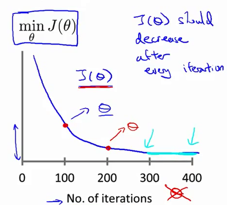
To check that gradient descent is working properly, we must verify the value of cost function J(theta) after each iteration.

So to each set of iterations , cost function J(theta) is decreasing and finally it converges to minimize and no more change like from 300 – 400.

Obvious gradient descent not working example

If our gradient descent graph shows like above, it means its not converging with each set of iteration and that means its not working properly. So in the above case, we can assume that alpha is pretty high, we must decrease the learning rate so that baby step would have taken.

·        For sufficiently small learning rate (alpha), J(theta) must decrease with every iteration.

·        But if learning rate is too small, gradient descent may take longer time to converge.

Conclusion:

·        Learning rate is too small, slow convergence.

·        Learning rate is too high, J(theta) may not converge or may not decrease with every iteration. It as well sometimes does slow convergence.

To choose try learning rate – 0.0001, 0.001, 0.01, 0.1, 1.. ….

Deciding Features (param) of a hypothesis\cost function

If we are given with multiple features (parameters), it always doesn’t make sense to use them as it is, we can do lots of other operations on it to make it better features.

Consider the following example-

So now as frontage * depth will give total area, we can derive-

x(land area) = frontage * depth

So now hypothesis,

h_Ɵ(x) = Ɵ₀ + Ɵ₁*x

So by defining new feature, we can define a new better model.